Weibull Analysis
– Reliability Life Data Analysis –

Introduction to Weibull Analysis
Almost every major item that consumers purchase has a warranty period. In most cases, you are encouraged by the seller to purchase an extended warranty or protection plan. Your first thought may be that if an extended warranty is needed, then this product is likely to fail just after the factory warranty has expired. It may cause you to doubt the quality of the product or questions how the warranty terms or the costs of extended warranties are determined. Warranty terms and conditions are generally based upon calculated risks of failure. Many companies and design engineers utilize a statistical tool called life data analysis otherwise known as Weibull Analysis. By determining the risk of a product or component failure, the manufacturer can better estimate warranty costs over time and assign a corresponding warranty period.
What is Weibull Analysis
Weibull Analysis is a methodology used for performing life data analysis. Life data is the result of measurements of a product’s life. Weibull Analysis is an effective method of determining reliability characteristics and trends of a population using a relatively small sample size of field or laboratory test data. Depending upon the product or industry, product life data is calculated in hours, miles, number of cycles or other metrics used to establish a measure of successful function of a product. The method is named for Mr. Waloddi Weibull who in 1937 invented the Weibull distribution. He presented a paper on the subject in 1951. Initial reaction to the paper initially ranged from uncertainty to total rejection. However, others in the field began to utilize and improve the method resulting in it being implemented by the U.S. Air Force in the 1970s, and later by the automotive industry. In industry today, Weibull Analysis is the foremost method for evaluating life data.
Types of Data
There are different types of life data and each type provides varying information regarding the product lifecycle. Analysis methods used vary according to the data type.
- Complete data: With Complete data, the practitioner is aware of the exact time-to-failure for a sample of the product. An example would be that the product failed at 15,000 cycles.
- Right Censored data: With Right Censored data, the practitioner successfully tests the product or component for a pre-determined or known period of time, number of cycles, etc. An example would be that the component operated successfully for 20,000 cycles. The product or component may have continued to perform within acceptable parameters for an unknown period.
- Interval data and Left Censored data: With these data types, the exact time-to-failure is unknown but it falls within a known time range. An interval is a defined length of time between two known points. Therefore, component failures between 10 and 50 hours of use represent interval data. If the component failures are between 0 and 50 hours, the data is considered left censored.
Probability Density Function
The Probability Density Function, or PDF, is used to determine the distribution of failures. The two commonly used versions of the Probability Density Function are the three-parameter PDF and two-parameter PDF. The three-parameter PDF examines:
- Shape, Threshold or Slope parameter, signified by the symbol b
- Scale or Characteristic Life parameter, signified by the symbol ƞ
- Location, Shift or Time to Failure parameter, signified by the symbol g
- This parameter is not included in the two-parameter PDF
The formulas for these Probability Density Functions can be found in the image to the right.
Although the calculations can be performed manually, there are various software packages and tools available to perform the calculations and generate the graphs. In the following example, a well-known software package was used.
The Shape Parameter
When the b value is represented on a graph, it is evident why it is termed the slope. The Shape Parameter is one of the most widely examined parameters because it helps indicate the types of failures occurring base on slope or the b value.
- If the value of b < 1, the failures will likely decrease over time. This could indicate a large number of infantile or early-life failures.
- A value of b = 1 indicates a constant failure rate which is indicative of the useful life or random failures.
- When the value of b > 1, the failure rate will generally increase over time. This could be an indication of premature wear issues, lack of proper maintenance or dictate the useful life of the product.
Why Perform Weibull Analysis
Most companies in business today monitor warranty costs and product failure rates. The goal is to reduce warranty costs and possible loss of brand equity. In addition, information gathered using a Weibull Analysis allows the manufacturer to plan for any known costs or set the proper warranty terms. Weibull Analysis is an effective method of determining reliability characteristics and trends of a population using a relatively small sample size of field or laboratory test data. Life data is the result of measurements of a product’s life. The Weibull Analysis is a valuable and relatively easy to apply tool that can be utilized by reliability engineers or analysts. The data set distribution may be used to evaluate product reliability, determine mean life, probability of failure at a specific time and estimate overall failure rates.
How to Perform Weibull Analysis
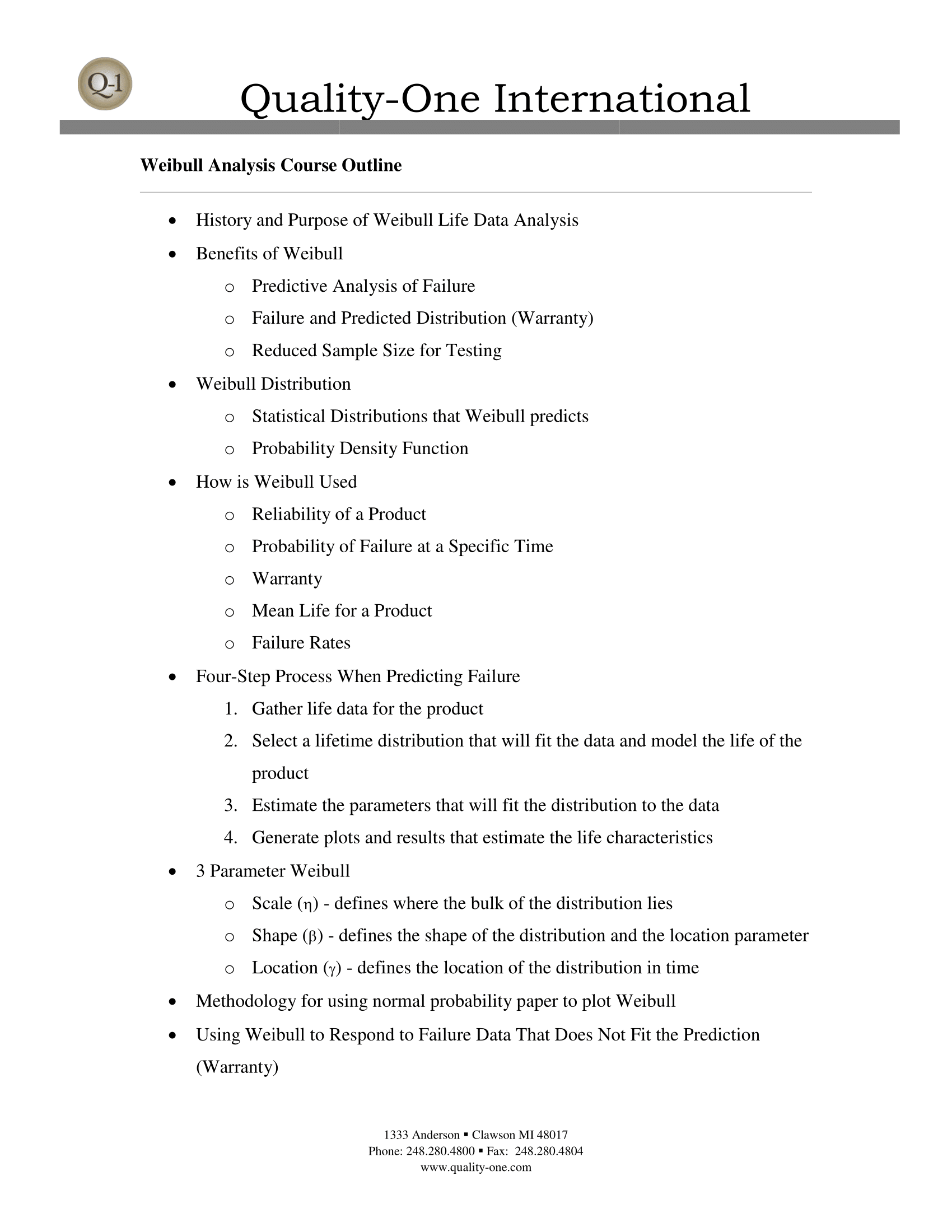
In previous sections, we reviewed some history of the Weibull Analysis, types of data, a definition of Weibull Analysis and why it is frequently used. In this section, we will investigate how to perform or complete a Weibull, or Life Data, Analysis. There are four main steps in performing a Weibull Analysis:
- Collect life data for a part or product and identify the type of data you are working with (Complete, Right Censored, Interval, Left Censored)
- Choose a lifetime distribution that fits the data and model the life of the part or product
- Determine the estimated parameters that will fit the distribution to the data
- Generate charts or plots that estimate the life characteristics for the part or product
Weibull Analysis Example
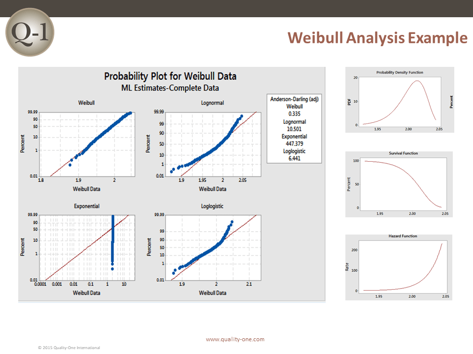
This example will analyze life data for motors in machinery currently in-use in the field. The unit performance is a function of running time in years. The first step is to examine the distribution ID plot of the data and select the line that best fits our data. Look for the lowest Anderson-Darling normality value. In addition, if the data follows a straight line and not concave when plotted on a log-log graph, the Weibull distribution can effectively describe the time to failure data. The lowest value indicates the data best fits a Weibull Analysis and the data also appears to fit the line in a straight line indicating that it can be described using a Weibull distribution.
The next step is to run a Probability Density Function (PDF) calculation and produce a corresponding graph. The PDF is a mathematical function that describes the distribution. It is similar to a histogram in that it illustrates the distribution of failure rates over a period time. The b, or slope value, is greater than 1 and the corresponding graph indicates that the failure rates are highest at about 2 years. This could be due to premature wear or indicate the expected life of the product. A thorough Root Cause Analysis (RCA) exercise should be completed to determine the cause or causes of failure, and work to resolve the problem.
There are other calculations that may also be performed and graphs generated to further examine the data set. A couple of examples are the Survival Function, represented by S (t), and the Hazard Function, represented by H (t).
- The Survival Function graph depicts the product’s chance of survival from introduction or in-service date until a specific time. Instead of looking for the proportion of product that will fail over time we examine the portion of product expected to survive.
- The Hazard Function graph depicts the rate of failure over a specified time. It is not a probability but a count of failures. This graph clearly indicates the point in time when the failures begin to rise and the percentage within a particular interval. In this example, it is clear that the rate of failures begins to rise dramatically between 2 and 2.05 years of use.
Several additional formulas and calculations are available to examine life data within the Weibull Analysis toolbox. This example focuses on the Probability Density Function and the Probability Plot of best fit to line exercise. Some examples of additional information that can be examined using a Weibull Analysis are listed below. This is a sample list and should not be considered a complete listing:
- Reliability at Specified Time: Calculates the likelihood that a product or component will still be operational at a particular point in time.
- Probability of Failure at Specified Time: Calculates the likelihood that a product or component will fail at a particular point in time. Probability of failure is sometimes called “unreliability”.
- Mean Life or Mean Time to Failure (MTTF): Denotes the average time in which the product or component are expected to operate successfully prior to failure. Also known as Mean Time Before Failure (MTBF).
- Rate of Failure: Indicates the quantity of product or component failures expected during a specified period of time.
- Reliable Life (warranty time): Estimated time when product reliability will be equivalent to a predetermined goal, such as 90% reliability. For example, it is estimated that 90% of the products in the field will be operational in 5 years.
The Weibull distribution is a versatile and powerful tool when applied and interpreted properly. It is frequently used to examine life data through the distributions parameters. During a Weibull Analysis we gather time to failure data, account for censored data, plot data and fit it to a line. During our analysis we also examine the slope of the line, which may provide clues to the type and source of the failures. The Weibull Analysis is an effective method to visualize and understand time to failure data. In addition, there are additional uses for the information derived from a Weibull analysis. Decisions can be made concerning the remaining product in the field regarding possible repair or replacement. In addition, the information can and should be utilized during New Product Introduction (NPI) projects or product improvement activities.
Weibull Analysis Services
At Quality-One, we will work with you to realize the full benefit of Weibull Analysis. Whether your goal is to understand the projected life or reliability of a product or gain insight into your current warranty costs, we can help. Our experienced team of highly trained professionals can develop a customized approach based on your unique needs. Whether you need Weibull Consulting plan, develop and implement the Weibull Analysis process, Weibull Training to bring your team up to speed or Weibull Support to assist with your current life data analysis projects, we are here to provide the service and expertise you need. At Quality-One, your success is our business!
Learn More About Weibull Analysis
Quality-One offers Quality and Reliability Support for Product and Process Development through Consulting, Training and Project Support. Quality-One provides Knowledge, Guidance and Direction in Quality and Reliability activities, tailored to your unique wants, needs and desires. Let us help you Discover the Value of Weibull Consulting, Weibull Training or Weibull Project Support.


